| threshold | sensitivity | precision |
|---|---|---|
| -1.62 | 50% | 50% |
| -1.25 | 30% | 91% |
| -0.38 | 10% | 100% |
| 0.23 | 5% | 100% |
| 0.74 | 1% | 100% |
| 1.30 | 0.1% | 100% |
buzzdetect sensitivity - how low can you go?
buzzdetect analysis
bioacoustics
Very low, as it turns out.
Overview
At the time of writing, the metrics for our best buzzdetect model are roughly 28% sensitivity at a 0.3% false positive rate, when calling detections with 95% precision. The corresponding threshold is -1.2; when the ins_buzz neuron is above -1.2, we consider the audio frame to be positive for insect flight activity.
-1.2 is a good starting point, but what if your results are really noisy? This happens when there is very little flight activity in your recordings. Our false positive rate is 0.3%, creating a noise floor that can swallow up trends. All hope is not lost - the distribution of neuron activations for true positives has a longer tail than that of of false positives, meaning we can still separate the two by increasing the detection threshold. The cost is that a high threshold rejects more true positives, decreasing our sensitivity. How low is too low for sensitivity? We’re starting at 28%, which is already a far cry from 100%, right? What’s the limit?
For better or for worse, the choice of threshold is subjective to the experiment in question. The right threshold is the one that maximizes the signal:noise ratio while preserving the trends of interest. Having to make a judgement call is, in one sense, a bummer. It would be nice to have one canonical number by which to call detections. The upside is freedom and rigor. Freedom because it allows flexbility in analysis, rigor because we can iterate and refine our analysis.
So: how low is too low?
TL;DR
Way low.
Worked examples
Let’s work with some real buzzdetect results to investigate this question. We’ll use the day-long results from the Five Flowers dataset, the same results we deposited with the buzzdetect manuscript (Figure 4) and the same ones used in the analysis walkthrough. We’ll only retain one recorder for each flower, so that we aren’t getting an overly-optimistic picture by averaging together results (thus boosting signal:noise). Then, we’ll apply a wide range of thresholds to the results and see how the trends change.
Choosing thresholds
We’ll use the following thresholds:
These thresholds span a wide range of sensitivity and precision. Threshold -1.62 is uselessly imprecise. -1.25 has a fairly usable precision of 91%, although in our experience that leads to visible false positives at night. The higher thresholds quickly saturate precision in the test set - 100% implies that all called buzzes were true buzzes. I’ll refer to these thresholds by their sensitivity values from now on, since the threshold value itself has no useful interpretation.
Trends in a single recorder in chicory
Let’s look at these thresholds when applied to our recorder in chicory.
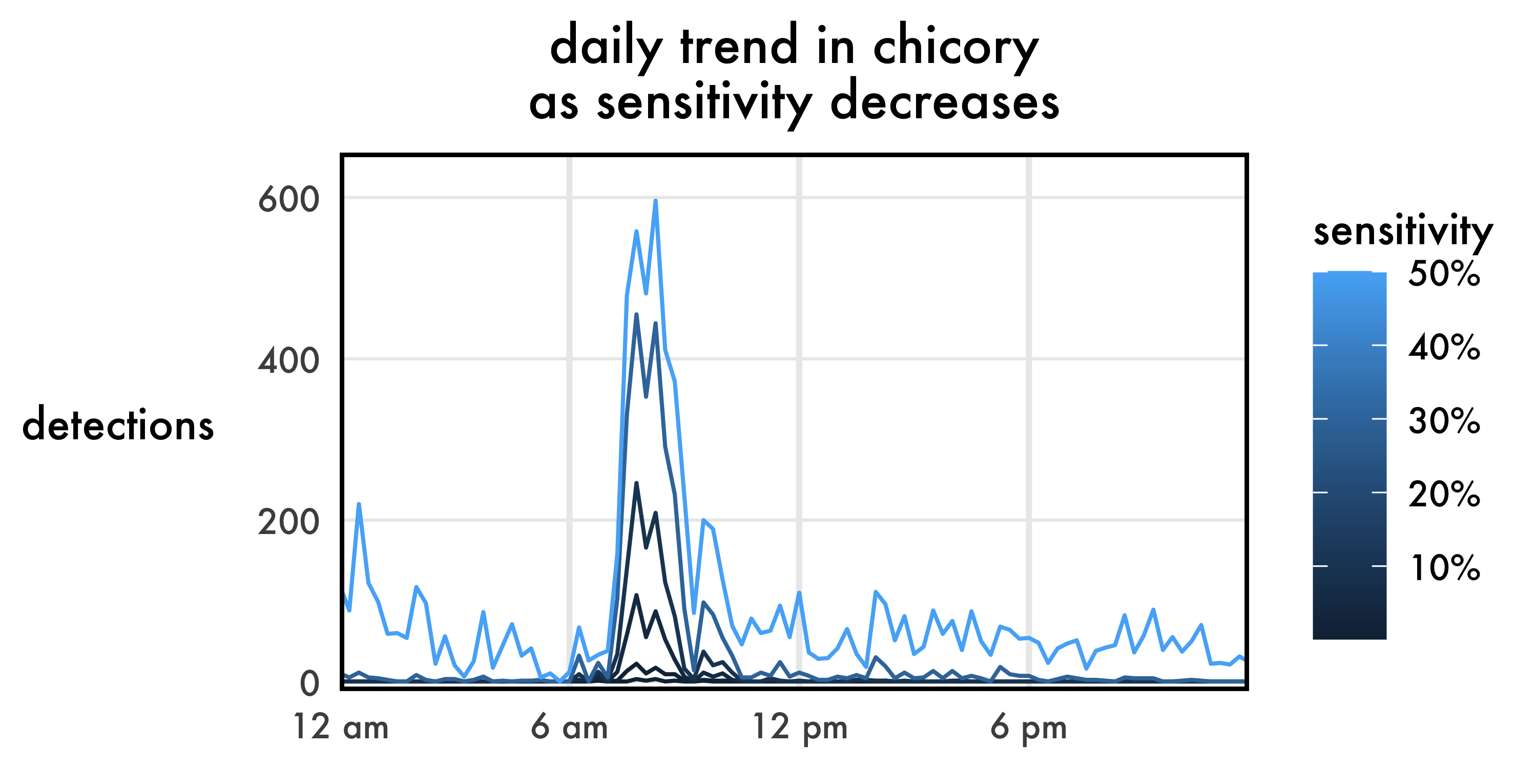
As expected, the low-precision results are way noisy. I somehow doubt there were 200 buzzes around 12:20 AM. But with a small step from 50% to 30% sensitivity, we go from 50% precision up to 91%, nearly completely removing the nighttime false positives. The daytime trend remains nearly identical, though of course with fewer total detections. It gets hard to see those darker lines as sensitivity plummets. On a common Y axis, they appear to show a similar, flatter trend? Let’s break out each line in its own panel with its own Y axis.
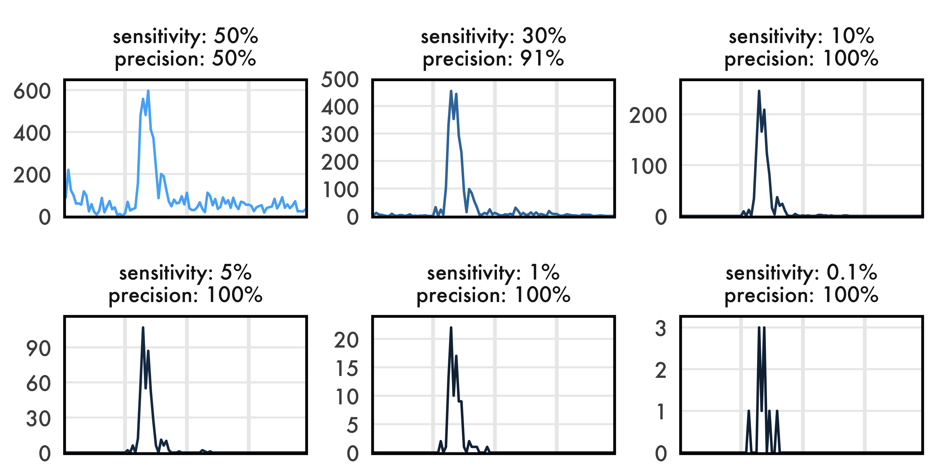
For the sake of space, I’m minimizing the axis text, but the axes are the same as the last plot - time of day on the X, detections on the Y. Note that the Y axis changes for each panel.
Interesting! Even though we’re dropping our sensitivity to nonsensical values, the overall trend is pretty much unaffected. The graph implies the same shape of the foraging curve, the same time of peak foraging, and roughly the same overall duration of foraging.
Looking at different flowers
Perhaps chicory is too easy. There’s a significant amount of foraging activity with a very tight diel pattern. That’s not always the case. Let’s bring in two more flowers. Mustard will serve as our high activity example. It has more bee activity than chicory (9,553 total detections vs 2,604) with sustained activity across the day. Watermelon will serve as the low-detections case (with a measly 335 detections).
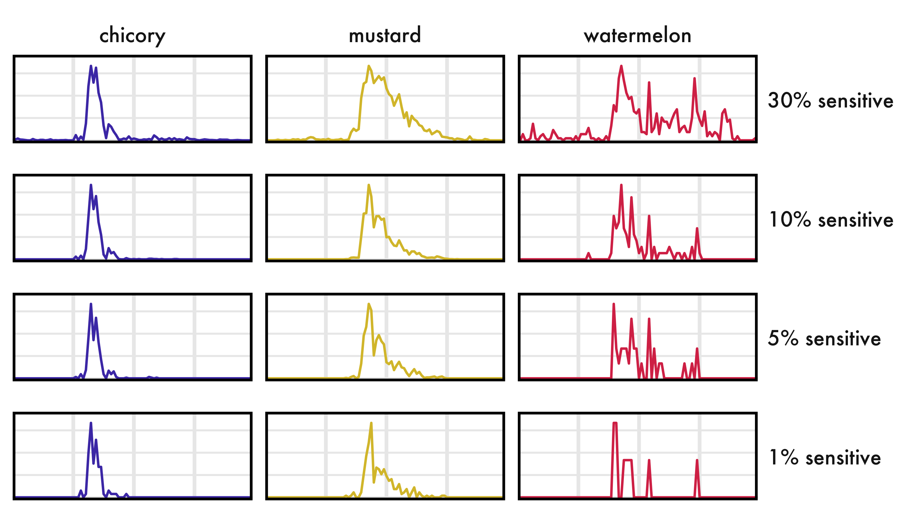
Again, I’m dropping a lot of axis text to make the trend clearer. The Y axis is detections, each panel scaled to fit the data. The X axis is still our full day.
A few observations:
- There are quite a few night detections in watermelon at 30% sensitivity (=91% precision). The other crops had the same threshold, but we don’t see the same number of night detections. What gives? In reality, watermelon doesn’t have more night positives. It has fewer! It only appears to have more nighttime detections than the other flowers because the peak detection rate is so low that it’s approaching the noise floor. Same threshold, same false positive rate (roughly), but a different precision because the underlying signal is weaker. This isn’t a model issue, or strictly a “flower” issue, it’s just the nature of the signal:noise beast.
- Where detections are low to begin with, the trend disappears more quickly. The curve for watermelon is significantly degraded at 1% sensitivity, while mustard remains largely the same from 10% through 1%.
- While the results are broad-strokes identical across reasonable sensitivities, some meaningful trends may still be affected by lower sensitivity. Take, for example, the daily pattern in mustard. Notice that the tail of foraging into the afternoon shrinks as sensitivity decreases. Those low detection rates later in the day get crushed to 0 as we crank threshold up. That could be a big deal if we’re interested in daily phenology! Maybe our statistical results wouldn’t be biased, because we might expect this effect to apply to all of our treatment groups. To my eye, though, chicory’s tight peak is less affected than mustard’s slow roll-off, which implies a differential effect from lowering sensitivity.
- It’s pretty wild that we get any trend at thresholds nearing 1%. Imagine doing field observations and letting 99 out of every 100 bees pass by without recording the observation. I think this is a testament to the sheer volume of bioacoustic data. There’s somewhere over 50,000 frames of audio in a summer day here in Ohio, producing substantially more detections than other observation methods even at ‘low’ sensitivity.
- It’s also downstream of the annotation/testing process. A bee might produce a buzz that covers 5 frames of buzz audio as it passes by the microphone. The middle frames would be loud, clear, and completely filled with buzzing. The first and last frames would be quiet, only partially contain buzzing, and would be slightly doppler-shifted as the bee approaches and leaves. We consider all five frames positive in the testing process if they contain at least 0.096s of buzzing. That’s a severely pessimistic estimate of sensitivity.